Introduction
In this blog we will run down the famous minimal character-level language model by Andrej Karpathy. The code has been modified to be supported by python 3. We will not only go through the code, but also look into the finer details of a RNN(Recurrent Neural Network) model. The explanation for the code can be found in the video lecture of CS231n 2016.
In this code, the objective is to model a sequence of text, and then predict characters. We can use absolutely anything as out input, lyrics of a song, \(\LaTeX\), python code and many more. In this blog I have used \(Rap God by Eminem\) to model upon. The lyrics has been taken from lyricfind.
Import
- Numpy
import numpy as np
Data I/O
This section deals with the data that will be input to the RNN model. The input.txt is a text file that is present as the input. The elements required as input:
- data - The input text
- chars - The unique characters of the input text
- char_to_ix - A dictionary that has a key value pair of unique characters to indices
- ix_to_char - A dictionary that has a key value pair of indices to unique characters
data = open('input.txt', 'r').read()
chars = list(set(data))
data_size, vocab_size = len(data), len(chars)
print('data has {} characters, {} unique.'.format(data_size, vocab_size))

char_to_ix = { ch:i for i,ch in enumerate(chars) }
ix_to_char = { i:ch for i,ch in enumerate(chars) }
data has 7855 characters, 64 unique.
Hyperparameters
The hyperparametes include:
- hidden_size - The hidden_size of the RNN cell
- seq_length - The length of sequence that is to be sampled.
- learning_rate - The learning rate serves as the coefficient of the updates.
hidden_size = 100 # size of hidden layer of neurons
seq_length = 50 # number of steps to unroll the RNN for
learning_rate = 1e-1
Model Parameters
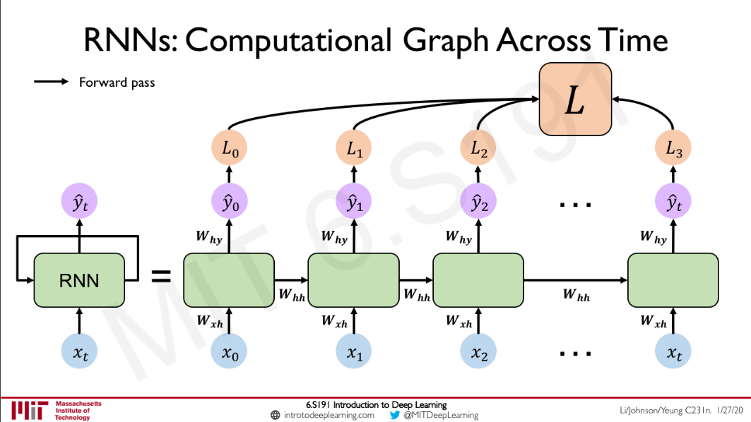
These are parameters that are important for the model. In a recurrent neural network, we have a hidden state that is calculated at each time step and fed to the next time step. The feed-forward part of a RNN model looks something like this  Source:Intro To Deep Learning \(h_{t} =f_{W}( h_{t-1} ,x_{t})\\ y_{t} =W_{hy} \times h_{t}\\\) The hidden state can be though of as the hidden layer of a vanilla deep neural network. The fact that makes RNNs awesome is the recurrence. The hidden state of previous time steps are fed to the present sequence models and this helps in the sequence modelling.
# model parameters
Wxh = np.random.randn(hidden_size, vocab_size)*0.01   # input to hidden
Whh = np.random.randn(hidden_size, hidden_size)*0.01  # hidden to hidden
Why = np.random.randn(vocab_size, hidden_size)*0.01   # hidden to output
bh = np.zeros((hidden_size, 1))                       # hidden bias
by = np.zeros((vocab_size, 1))                        # output bias
Loss Function
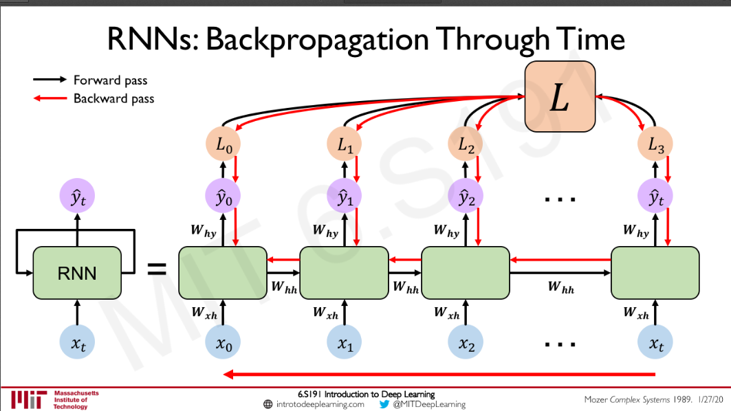
In this section we will look into the loss function of the model. The objective of our problem is to model language in a character level scheme. The model should be able to predict a character that come after a given sequence of characters. We use the softmax loss \(\boxed{p_{k} =\frac{e^{f_{k}}}{\sum _{j} e^{f_{j}}}}\\ \mathcal{L}_{i} =-\log p_{y_{i}}\\ \Longrightarrow \mathcal{L}_{i} =-\log\frac{e^{f_{y_{i}}}}{\sum _{j} e^{f_{j}}}\\ \Longrightarrow \mathcal{L}_{i} =-\log e^{f_{y_{i}}} +\log\sum _{j} e^{f_{j}}\\ \Longrightarrow \boxed{\mathcal{L}_{i} =-f_{y_{i}} +\log\sum _{j} e^{f_{j}}}\) I would like to make you all understand the back-propagation of the \(\mathcal{L}_{i}\) too. There are two conditions of the back-propagation.
- The part where \(\displaystyle k=y_{i}\) \(\frac{\partial \mathcal{L}_{i}}{\partial f_{k}} =\frac{\partial \left( -f_{y_{i}} +\log\sum _{j} e^{f_{j}}\right)}{\partial f_{k}}\\ \Longrightarrow \frac{\partial \mathcal{L}_{i}}{\partial f_{k}} =-1+\frac{\partial \log\sum _{j} e^{f_{j}}}{\partial f_{k}}\\ \Longrightarrow \frac{\partial \mathcal{L}_{i}}{\partial f_{k}} =-1+\frac{\partial \log\sum _{j} e^{f_{j}}}{\partial \sum _{j} e^{f_{j}}}\frac{\partial \sum _{j} e^{f_{j}}}{\partial f_{k}}\\ \Longrightarrow \frac{\partial \mathcal{L}_{i}}{\partial f_{k}} =-1+\frac{1}{\sum _{j} e^{f_{j}}} e^{f_{y_{i}}}\\ \Longrightarrow \frac{\partial \mathcal{L}_{i}}{\partial f_{k}} =-1+\frac{e^{f_{y_{i}}}}{\sum _{j} e^{f_{j}}}\\ \Longrightarrow \boxed{\frac{\partial \mathcal{L}_{i}}{\partial f_{k}} =-1+p_{y_{i}}}\)
- The part where \(\displaystyle k\neq y_{i}\) \(\frac{\partial \mathcal{L}_{i}}{\partial f_{k}} =\frac{\partial \left( -f_{y_{i}} +\log\sum _{j} e^{f_{j}}\right)}{\partial f_{k}}\\ \Longrightarrow \frac{\partial \mathcal{L}_{i}}{\partial f_{k}} =\frac{\partial \log\sum _{j} e^{f_{j}}}{\partial f_{k}}\\ \Longrightarrow \frac{\partial \mathcal{L}_{i}}{\partial f_{k}} =\frac{\partial \log\sum _{j} e^{f_{j}}}{\partial \sum _{j} e^{f_{j}}}\frac{\partial \sum _{j} e^{f_{j}}}{\partial f_{k}}\\ \Longrightarrow \frac{\partial \mathcal{L}_{i}}{\partial f_{k}} =\frac{1}{\sum _{j} e^{f_{j}}} e^{f_{k}}\\ \Longrightarrow \frac{\partial \mathcal{L}_{i}}{\partial f_{k}} =\frac{e^{f_{k}}}{\sum _{j} e^{f_{j}}}\\ \Longrightarrow \boxed{\frac{\partial \mathcal{L}_{i}}{\partial f_{k}} =p_{k}}\)
To simplify the whole gradient we can rewrite it as: \(\boxed{\frac{\partial \mathcal{L}_{i}}{\partial f_{k}} =p_{k} -\ \mathbb{1}( k=y_{i})}\)  Source:Intro To Deep Learning
def lossFun(inputs, targets, hprev):
    """
    inputs,targets are both list of integers.
    hprev is Hx1 array of initial hidden state
    returns the loss, gradients on model parameters, and last hidden state
    """
    xs, hs, ys, ps = {}, {}, {}, {}
    hs[-1] = np.copy(hprev)
    loss = 0

    # forward pass
    for t in range(len(inputs)):
        xs[t] = np.zeros((vocab_size,1)) # encode in 1-of-k representation
        xs[t][inputs[t]] = 1

        hs[t] = np.tanh(np.dot(Wxh, xs[t]) + np.dot(Whh, hs[t-1]) + bh) # hidden state
        ys[t] = np.dot(Why, hs[t]) + by # unnormalized log probabilities for next chars
        ps[t] = np.exp(ys[t]) / np.sum(np.exp(ys[t])) # probabilities for next chars
        loss += -np.log(ps[t][targets[t],0]) # softmax (cross-entropy loss)

    # backward pass: compute gradients going backwards
    dWxh, dWhh, dWhy = np.zeros_like(Wxh), np.zeros_like(Whh), np.zeros_like(Why)
    dbh, dby = np.zeros_like(bh), np.zeros_like(by)
    dhnext = np.zeros_like(hs[0])
    for t in reversed(range(len(inputs))):
        dy = np.copy(ps[t])
        dy[targets[t]] -= 1

        dWhy += np.dot(dy, hs[t].T)
        dby += dy
        dh = np.dot(Why.T, dy) + dhnext # backprop into h
        dhraw = (1 - hs[t] * hs[t]) * dh # backprop through tanh nonlinearity
        dbh += dhraw
        dWxh += np.dot(dhraw, xs[t].T)
        dWhh += np.dot(dhraw, hs[t-1].T)
        dhnext = np.dot(Whh.T, dhraw)
    for dparam in [dWxh, dWhh, dWhy, dbh, dby]:
        np.clip(dparam, -5, 5, out=dparam) # clip to mitigate exploding gradients
    return loss, dWxh, dWhh, dWhy, dbh, dby, hs[len(inputs)-1]
def sample(h, seed_ix, n):
    """
    sample a sequence of integers from the model
    h is memory state, seed_ix is seed letter for first time step
    n is the number of charaters that we want to predict
    """
    # To one hot encode the seed
    x = np.zeros((vocab_size, 1))
    x[seed_ix] = 1

    ixes = []
    for t in range(n):
        h = np.tanh(np.dot(Wxh, x) + np.dot(Whh, h) + bh)
        y = np.dot(Why, h) + by
        p = np.exp(y) / np.sum(np.exp(y))
        ix = np.random.choice(range(vocab_size), p=p.ravel())
        # The one hot encoding of the character predicted
        x = np.zeros((vocab_size, 1))
        x[ix] = 1
        ixes.append(ix)
    return ixes
# n - iteration counter
# p - move data pointer
n, p = 0, 0

# Memory variables for Adagrad Update:
mWxh, mWhh, mWhy = np.zeros_like(Wxh), np.zeros_like(Whh), np.zeros_like(Why)
mbh, mby = np.zeros_like(bh), np.zeros_like(by)

smooth_loss = -np.log(1.0/vocab_size)*seq_length # loss at iteration 0
for i in range(20000):
    # prepare inputs (we're sweeping from left to right in steps seq_length long)
    if p+seq_length+1 >= len(data) or n == 0:
        hprev = np.zeros((hidden_size,1)) # reset RNN memory
        p = 0 # go from start of data
    inputs = [char_to_ix[ch] for ch in data[p:p+seq_length]]
    targets = [char_to_ix[ch] for ch in data[p+1:p+seq_length+1]]

    # sample from the model now and then
    if n % 5000 == 0:
        sample_ix = sample(hprev, inputs[0], 200)
        txt = ''.join(ix_to_char[ix] for ix in sample_ix)
        print('----\n {} \n----'.format(txt))

    # forward seq_length characters through the net and fetch gradient
    loss, dWxh, dWhh, dWhy, dbh, dby, hprev = lossFun(inputs, targets, hprev)
    smooth_loss = smooth_loss * 0.999 + loss * 0.001
    if n % 100 == 0: print('iter {}, loss: {:0.2f}'.format(n, smooth_loss)) # print progress

    # perform parameter update with Adagrad
    for param, dparam, mem in zip([Wxh, Whh, Why, bh, by],
                                  [dWxh, dWhh, dWhy, dbh, dby],
                                  [mWxh, mWhh, mWhy, mbh, mby]):
        mem += dparam * dparam
        param += -learning_rate * dparam / np.sqrt(mem + 1e-8) # adagrad update

    p += seq_length # move data pointer
    n += 1 # iteration counter
----
u'KG"iWIn4uyZx YWOFAeE2dNcDeId!7Zdrs2veTFOCR"hsc7HUd2n"y/P-22DcrRpZY,d/'tb?Z(vwcgUnll,vDE/?ifjH.UhzG..KEmMxtA
eEC' BGLPOaTttouWETM/z!,pF.(A muIsABRA'2
sMREIKt
C0

kAslfib.FPZuHFd
ryum.DO-2nZ!mGriHpZ.G
----
iter 0, loss: 207.94
iter 100, loss: 207.71
.
.
.
iter 4900, loss: 104.81
----
y's jucs, ohing the im ind Ret's may I din Yehingeverd, reve goinrithe, Dust to thatyo I may,rer it bomow sou tos as 'lnop, I hoardy thor coune otere
'Cs at tinn to rust a then
KI'mid?
A0d, etey
Wy ho
----
iter 5000, loss: 103.99
.
.
.
iter 9900, loss: 77.70
----
ap to' chere I'm ansibple hinot fron make the feill tho bevcat
I'd stth thet ould
OnOd
All ca
Rat mang ther at ffom will
But they samas
Son wank yo
Merthent flo I'm sthe thibe whot arla ct an onthy ho
----
iter 10000, loss: 77.42

iter 14900, loss: 69.94
----
 hot ag
Andad the ly-wang, doont bas a lake sough thumal
Ass bas ibuth ike whey poc, Helike akp hock Fy?
Ang a ken peryous
I'm a grime, D-bo ourd not song' noig't ang thens procly, you
So noont wen hu
----
iter 15000, loss: 69.14
iter 15100, loss: 68.69
iter 15200, loss: 68.01
.
.
.
----
I gale able ono the think is wicty
Withure's singe
Se'll, mall nay home likn at a fut, and armating I king deapee besly chacaus louly bomh
And arsiting thatow a nelis at ane I a chat tod a simakend a
----
Conclusion
This was a quick tour of all the code written by Andrej Karpaty. I would definitely want you all to run the code and do some crazy stuff with this.