In a neural network, the weights and biases that correspond to individual neurons are the only variables. They change and try reaching an optimum stage where the whole model seems to make good predictions on the given data. With an optimum configuration of the weights and biases each neuron fires differently for a particular data point.
This notebook is based on a thought experiment. While making a classification model, does the model’s neurons fire similarly for similar classes?
Here I am interested in looking at the pattern of neuron activation for individual classes. After that, I would try drawing a parallel between classes with similar activation patterns.
The data-set that has been worked upon is the Fashion MNIST. The classification task was to correctly classify each of the 10 classes. The neuron activation pattern has been noted and then later correlated.
Imports
Import the important packages.
import numpy as np
import tensorflow as tf
from tensorflow import keras
import matplotlib.pyplot as plt
%matplotlib inline
print(tf.__version__)
2.2.0
(X_train, y_train), (X_test, y_test) = keras.datasets.fashion_mnist.load_data()
X_train.shape
(60000, 28, 28)
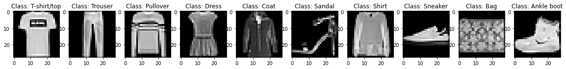
There are 60,000 images in the data-set. There are 10 classes as mentioned below. Each of the class has 6,000 samples. The images are 28x28 pixels and have 1 channel. 1 channel refers to the fact that each and every image has only the gray channel to express its colour.
The Data-set
Let us see the data and get familiar with it. The 10 classes in the F-MNIST data-set are as follows:
- T-shirt/top
- Trouser
- Pullover
- Dress
- Coat
- Sandal
- Shirt
- Sneaker
- Bag
- Ankle boot
class_names = {
    0:	'T-shirt/top',
    1: 	'Trouser',
    2: 	'Pullover',
    3: 	'Dress',
    4: 	'Coat',
    5: 	'Sandal',
    6: 	'Shirt',
    7: 	'Sneaker',
    8: 	'Bag',
    9:  'Ankle boot'
}
plt.figure(figsize=(20,10))
for i in range(10):
  plt.subplot(1,10,i+1)
  plt.imshow(X_train[y_train == i][0],cmap='gray')
  plt.title('Class: {}'.format(class_names[i]))
Preprocess the Data
This is a little step that needs to be performed before entering the next step. If we went ahead and looked into the shape of a single image from the data-set we would see that it has a dimension of (28, 28). This can be thought of as a 2 dimensional matrix with 28 rows and 28 columns where each individual element is the pixel value at that position. This makes sense right? Yeah it does, but this is not it. As I had previously mentioned about the channel, we need to specify that information here. We need to convert each image from (28, 28) to (28, 28, 1). This does not create a whole lot of difference, but later when we have more channels like in coloured images (3 channels namely Red, Green, Blue) we would require them to have a 3 dimensional array. To keep parity in the way we work and due to the fact that the tf.keras convolution API takes a 3 dimensional image, the preprocessing is important.
X_train = X_train.reshape(60000,28,28,1)
X_test = X_test.reshape(10000,28,28,1)
print('X_train shape {}'.format(X_train.shape))
print('X_test shape {}'.format(X_test.shape))
X_train shape (60000, 28, 28, 1) X_test shape (10000, 28, 28, 1)
Here we one-hot encode the class labels.
y_train_one_hot = tf.keras.utils.to_categorical(y_train, 10)
y_test_one_hot = tf.keras.utils.to_categorical(y_test, 10)
print('y_train_one_hot shape {}'.format(y_train_one_hot.shape))
print('y_test_one_hot shape {}'.format(y_test_one_hot.shape))
y_train_one_hot shape (60000, 10) y_test_one_hot shape (10000, 10)
Model
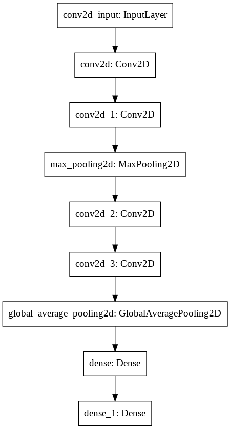
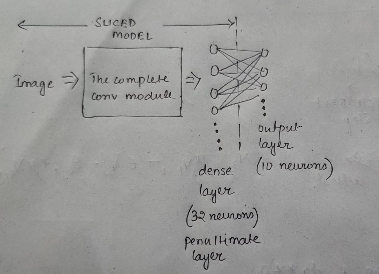
The model is relatively simple. I have summarised the model below and have also drew out the model image for better understanding.
model = tf.keras.models.Sequential()
model.add(tf.keras.layers.Conv2D(filters=32,
                                 kernel_size=(3,3),
                                 activation='relu',
                                 input_shape =(28,28,1)))
model.add(tf.keras.layers.Conv2D(filters=32,
                                 kernel_size=(3,3),
                                 activation='relu'))
model.add(tf.keras.layers.MaxPool2D(pool_size=(2,2)))

model.add(tf.keras.layers.Conv2D(filters=64,
                                 kernel_size=(3,3),
                                 activation='relu'))
model.add(tf.keras.layers.Conv2D(filters=64,
                                 kernel_size=(3,3),
                                 activation='relu'))

model.add(tf.keras.layers.GlobalAveragePooling2D())
model.add(tf.keras.layers.Dense(units=32, activation='relu'))
model.add(tf.keras.layers.Dense(units=10, activation='softmax'))
model.summary()
Model: "sequential"
_________________________________________________________________
Layer (type)                 Output Shape              Param #
=================================================================
conv2d (Conv2D)              (None, 26, 26, 32)        320
_________________________________________________________________
conv2d_1 (Conv2D)            (None, 24, 24, 32)        9248
_________________________________________________________________
max_pooling2d (MaxPooling2D) (None, 12, 12, 32)        0
_________________________________________________________________
conv2d_2 (Conv2D)            (None, 10, 10, 64)        18496
_________________________________________________________________
conv2d_3 (Conv2D)            (None, 8, 8, 64)          36928
_________________________________________________________________
global_average_pooling2d (Gl (None, 64)                0
_________________________________________________________________
dense (Dense)                (None, 32)                2080
_________________________________________________________________
dense_1 (Dense)              (None, 10)                330
=================================================================
Total params: 67,402
Trainable params: 67,402
Non-trainable params: 0
_________________________________________________________________
tf.keras.utils.plot_model(
    model,
    to_file="model.png"
)
Training
At this step we train the model to fit on out Fashion MNIST dat-aset.
tf.keras.backend.clear_session()
model.compile(
    optimizer='adam', loss='categorical_crossentropy', metrics=['acc']
)
history = model.fit(
    x=X_train,
    y=y_train_one_hot,
    validation_split=0.3,
    batch_size=32,
    epochs=15
)
Epoch 1/15
1313/1313 [==============================] - 6s 4ms/step - loss: 0.6822 - acc: 0.7552 - val_loss: 0.5710 - val_acc: 0.7761
Epoch 2/15
1313/1313 [==============================] - 6s 4ms/step - loss: 0.4316 - acc: 0.8446 - val_loss: 0.4248 - val_acc: 0.8445
Epoch 3/15
1313/1313 [==============================] - 6s 4ms/step - loss: 0.3564 - acc: 0.8726 - val_loss: 0.3293 - val_acc: 0.8816
Epoch 4/15
1313/1313 [==============================] - 6s 4ms/step - loss: 0.3174 - acc: 0.8870 - val_loss: 0.3248 - val_acc: 0.8836
Epoch 5/15
1313/1313 [==============================] - 6s 4ms/step - loss: 0.2877 - acc: 0.8952 - val_loss: 0.2783 - val_acc: 0.9014
Epoch 6/15
1313/1313 [==============================] - 6s 4ms/step - loss: 0.2590 - acc: 0.9063 - val_loss: 0.2826 - val_acc: 0.8992
Epoch 7/15
1313/1313 [==============================] - 6s 4ms/step - loss: 0.2421 - acc: 0.9112 - val_loss: 0.3085 - val_acc: 0.8929
Epoch 8/15
1313/1313 [==============================] - 6s 4ms/step - loss: 0.2235 - acc: 0.9190 - val_loss: 0.2687 - val_acc: 0.9042
Epoch 9/15
1313/1313 [==============================] - 6s 4ms/step - loss: 0.2082 - acc: 0.9227 - val_loss: 0.2600 - val_acc: 0.9072
Epoch 10/15
1313/1313 [==============================] - 6s 4ms/step - loss: 0.1917 - acc: 0.9302 - val_loss: 0.2714 - val_acc: 0.9038
Epoch 11/15
1313/1313 [==============================] - 6s 4ms/step - loss: 0.1785 - acc: 0.9358 - val_loss: 0.2690 - val_acc: 0.9068
Epoch 12/15
1313/1313 [==============================] - 6s 4ms/step - loss: 0.1679 - acc: 0.9380 - val_loss: 0.2884 - val_acc: 0.9025
Epoch 13/15
1313/1313 [==============================] - 6s 4ms/step - loss: 0.1526 - acc: 0.9442 - val_loss: 0.2656 - val_acc: 0.9108
Epoch 14/15
1313/1313 [==============================] - 6s 4ms/step - loss: 0.1425 - acc: 0.9482 - val_loss: 0.2873 - val_acc: 0.9068
Epoch 15/15
1313/1313 [==============================] - 6s 4ms/step - loss: 0.1349 - acc: 0.9505 - val_loss: 0.2873 - val_acc: 0.9067
Model History
This is just the code snippet to see the training graphs of the model. The training accuracy and the validation accuracy have been logged jointly in one plot. On the other plot the training loss and the validation loss have been logged.
plt.subplot(2,1,1)
# summarize history for accuracy
plt.plot(history.history['acc'])
plt.plot(history.history['val_acc'])
plt.title('model accuracy')
plt.ylabel('accuracy')
plt.xlabel('epoch')
plt.legend(['train', 'test'], loc='upper left')
plt.show()
plt.subplot(2,1,2)
# summarize history for loss
plt.plot(history.history['loss'])
plt.plot(history.history['val_loss'])
plt.title('model loss')
plt.ylabel('loss')
plt.xlabel('epoch')
plt.legend(['train', 'test'], loc='upper left')
plt.show()
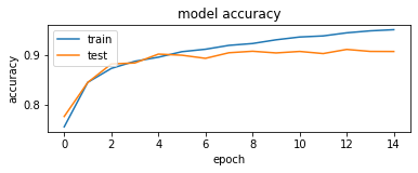
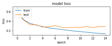
The graphs do show that the models indeed converge and are picking up on the learning aspect.
model.evaluate(X_test, y_test_one_hot)
313/313 [==============================] - 1s 2ms/step - loss: 0.3204 - acc: 0.9044 [0.3203956186771393, 0.9043999910354614]
The model does pretty well with a loss of 0.32 and an accuracy of 0.90
Slice the model
We have seen that the model did fairly well on the unseen test data. Now we would look into the pattern of activation of neurons in the penultimate layer of the model. There was not particular reason behind my choosing this particular layer. Here the penultimate layer is named as dense. The penultimate layer has 32 neurons.
So we would pass in 1000 examples of each individual class and keep track of the pattern of neurons firing.
layer_name = 'dense' #Name of the penultimate layer.
intermediate_layer_model = tf.keras.Model(inputs=model.input,
                                 outputs=model.get_layer(layer_name).output)
Experiment
Let us talk about the experiment. I have a classification model that classifies images that are fed to it. My hypothesis is that different neurons fire (activate) for different classes. The activation of the neurons must bare a pattern along them, similar classes must have similar neurons getting activated.
The model is sliced till the layer that is to be observed (here it is the penultimate “dense” layer). The penultimate layer has 32 neurons that have ReLU activation function. So they either activate and provide a positive value or else do not activate at all. To make things simple I have turned all positive numbers to 1. So now we can think for a neuron either activating and producing a 1 or not activating and producing a 0.
The methodology of the experiment is to provide 1000 samples from each individual class to test and note the activation pattern of each of the 32 neurons. Later, the neuron activations for each class becomes the base of correlation.
class_vs_neurons = np.zeros((10,32))
for idx in range(10):
  class_choice = X_test[y_test == idx]
  intermediate_output = intermediate_layer_model.predict(class_choice)
  intermediate_output[intermediate_output > 0] = 1.0
  class_vs_neurons[idx,:] = np.sum(intermediate_output,axis=0)/1000
Look for similar patterns of neuron activation
Similarity in activation of neurons is quantified by calculating the difference between the activations for classes. This way each of the class activation pattern is correlated with every other class activation.
corr = np.zeros((10,10))
for i in range(10):
  for j in range(10):
    corr[i,j] = np.sum(np.absolute(class_vs_neurons[i] - class_vs_neurons[j]))/32
plt.figure(figsize=(10,20))
for i in range(10):
  idx_sort = corr[i].argsort()
  for j in range(10):
    plt.subplot(10,10,10*i+j+1)
    plt.imshow(X_train[y_train == idx_sort[j]][0].reshape(28,28), cmap='gray')
    plt.xticks([])
    plt.yticks([])
plt.show()
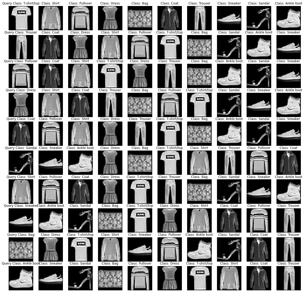
The above image is presented in a particular way. The reader is supposed to look at the rows from left to right. In each row, the first image is the queried class, the following images are arranged according to their similarities of neuron activation for the particular class. Here one can notice similar classes like t-shirt, shirt and pullovers are close to each other while sandlas, sneakers and ankle-boots are grouped together. The image is conclusive of the fact that similar classes indeed fire similar neurons.
I am new to deep learning and would really love the inputs from other people. I would also love constructive feedbacks on the experiment.